H2O Tree API - Inspecting trees in H2O
H2O-3, the open source machine learning platform offers several algorithms based on decision trees. In latest stable release, we’ve made it possible for data scientists and developers to inspect the trees thoroughly. We’ve created unified API to access every single tree in all tree-based algorithms available in H2O, namely:
In addition, algorithms like GBM or XGBoost may be part of Stacked Ensembles models or leveraged by AutoML. As a part of H2O’s strategy of explainable AI, an API has been built to allow data scientists inspect decision trees built while training the above-mentioned algorithms. A complete version of this API with support for all the algorithms is available since version 3.22.0.1, codename xia (named after Zhihong Xia. There is a user guide with instructions on how to install the newest version of H2O available on H2O documentation page.
This guide is for advanced H2O users. For beginners, there is an introductionary article named Machine Learning With H2O — Hands-On Guide for Data Scientists.
H2O Tree API overview
H2O tree-based algorithms produce many trees during the training process. The ability to fetch and inspect each tree separately is a crucial part of the API. No tree is lost. As long as a model is not deleted trees can be fetched using Python and R.
Obtaining a tree is a matter of a single API call both in Python
1
2
from h2o.tree import H2OTree
tree = H2OTree(model = airlines_model, tree_number = 0, tree_class = None)
and in R.
1
  tree <- h2o.getModelTree(model = airlines.model, tree_number = 1, tree_class = "NO")
There is nothing more to fetching a tree. However, the internal structure of the objects fetched is rich & fun to explore. It contains all the information available about every node in the graph. It provides both human-readable output and format suitable for machine processing.
In the fetched object, there two representations of the graph contained:
- graph-oriented representation, starting with a root node with edges,
- array/vector representation, useful for quick machine processing of the tree’s structure.
At tree level, the following information is provided:
- Number of nodes in the tree,
- Model the tree belongs to,
- Tree class (if applicable),
- Pointer to a root node for tree traversal (breadth-first, depth-first) and manual tree walking.
Each node in the tree is uniquely identified by an ID, regardless of its type. Also for each node type, a human-redable description is available. There are two types nodes distinguished:
- Split node,
- Leaf node.
A split node is a single non-terminal node with either numerical or categorical feature split. The root node is guaranteed to be a split node, as a zero-depth tree t of cardinality |t| = 1 contains no decisions at all. Split node consists of:
- H2O-specific node identifier (ID - all nodes have it),
- Left child node & right child node,
- Split feature name (split column name),
- Split threshold (mainly for numerical splits),
- Categorical features split (categorical splits only),
- Direction of NA values (which way NA values go - left child, right child or nowhere).
A leaf node is a single node with no children, thus being a terminal node at the end of the decision path in a tree. Leaf node consists of:
- H2O-specific node identifier (ID - all nodes have it),
- Prediction value (floating point number).
How to fetch the tree, distinguish between node types & obtain information about nodes is demonstrated in the next two sections. One section dedicated to Python API and the other dedicated to R API. Both sections are identical in content, as both APIs provide the same functionality, only the API used is different.
Python client
As an example dataset, a widely-known Airlines Delay dataset is used. All the example scripts will automatically download the dataset, thus there is no need to download it in advance.
To fetch a tree from a decision tree-based model, it is required to build the model. All the machine learning algorithms with a decision trees as an output are supported. For demonstration purpose, GBM is chosen. It can be found in h2o.estimators package. The fully qualified name of GBM is h2o.estimators.gbm.H2OGradientBoostingEstimator. The approach to obtain trees for all the algorithms is exactly the same. Simply substituting GBM model with DRF, XGBoost or any other supported algorithm is going to work flawlessly.
Building the example model
Goal is not to produce the best predictor, but an understandable one. Therefore, the example GBM model is very simple. The following script connects H2O Python client to H2O backend and imports the Airlines dataset. As GBM has been chosen, H2OGradientBoostingEstimator is imported from h2o.estimators package to avoid addressing the GBM estimator by its fully qualified name all the time. To keep the model training time at minimum, a maximum number of trees is limited to 3. In order to make the decision tree small and easily understandable, maximum depth of the decision tree is limited to 3. As the tree is binary, this is going to limit the number of nodes to 7. A root node with two children, plus maximum of two children per each of root node’s children. This leads to a total of 7 nodes.
1
2
3
4
5
6
import h2o
h2o.init()
airlines_data = h2o.import_file("https://s3.amazonaws.com/h2o-airlines-unpacked/allyears2k.csv")
from h2o.estimators import H2OGradientBoostingEstimator
airlines_gbm_model = H2OGradientBoostingEstimator(ntrees = 3, max_depth = 2)
airlines_gbm_model.train(x = ["Origin"], y = "Distance", training_frame = airlines_data)
Fetching a basic tree
As the model that is trying to guess the distance of a flight based on flight’s origin is built, the only next step required is to fetch the decision trees behind it. The only next step is to fetch the actual tree. The number of trees in the model has been set to 3 in the H2OGradientBoostingEstimator’s parameters. This means there are three trees to be fetched. When training real models, always watch for early stopping criteria. Having those in place may result in even fewer trees trained than set in the ntrees argument of H2OGradientBoostingEstimator’s constructor.
A tree in H2O’s Python API is represented by a class named H2OTree and is placed in a package h2o.tree. Its fully qualified name is h2o.tree.H2OTree. As a sidenote for Python users also interested in R, the class name H2OTree is shared with R API. An instance of H2OTree represents a single tree related to a single model. If there are n trees built during the training process of a model, then n instances of H2OTree class must be created represent the full set. A tree is fetched by means of H2OTree’s constructor. It takes three arguments:
- Model to fetch the tree from,
- Ordinal number of the tree to fetch
- Class of the tree to fetch
The very first argument is the model. The variable pointing to the GBM model is airlines_gbm_model (as shown in the figure above). As the model is training is progressing, multiple trees are built. The second arguments specifies which tree we’d like to build. In Python, indices are numebered from 0, so the index of the first tree is 0 as well. The number of trees has been limited to 3 in the example. For a real-world model, the number of trees behind it can be obtained by accessing the ntrees field of the model, in this case airlines_gbm_model.ntrees. The last argument specifies the class of the tree. This argument only applies to categorial response variables. This is not the case of the airlines_gbm_model, which has Distance set as a response variable. Distance’s type is numeric, thus the problem is a regression and the class is simply None. In case of binomial and multinomial models, the class must be specified. Tree classes correspond to the categorical levels of response variable. Fetching of models with categorical response variable is demonstrated in one of the sections below, accompanied with full explanation.
1
2
from h2o.tree import H2OTree
first_tree = H2OTree(model = airlines_gbm_model, tree_number = 0, tree_class = None)
By issuing the commands in the figure above, a tree is fetched and an instance of H2OTree is created. The tree is related to airlines_gbm_model, it is the very first tree created and due to the nature of the problem (regression), there is no tree class.
Exploring a basic tree
The H2OTree contains all the information available for given tree. A very basic task is to find out how many nodes are there in the tree. Giving the first_tree as an argument to Python’s built-in len function provides the answer.
1
2
len(first_tree)
7
Another basic task before tree nodes exploration would be printing general description of a tree. To achieve this, give first_tree as an argument to Python’s built-in print function.
1
2
print(first_tree)
Tree related to model GBM_model_python_1537893605654_1. Tree number is 0, tree class is 'None'
The H2OTree type has a lot of properties:
- left_children,
- right_children,
- node_ids,
- descriptions,
- model_id,
- tree_number,
- tree_class,
- thresholds,
- features,
- levels,
- nas,
- predictions,
- root_node.
The properties tree_number, tree_class and model_id were present in print(first_tree)’s output. These are related to the tree’s model and together serve a H2OTree's unique identifier. In the next figure, content of those three properties is demonstrated separately.
As mentioned in the introductionary chapter, there are array-like structures for fast iteration through the tree. There is also a pre-built tree structure to walk. As every tree begins with a root node, the root_node property of type H2ONode serves as an entry point to the tree. Besides having several properties to inspect, it also points to its child nodes. Same rules apply to all other nodes when walking down any path in the graph, unless a terminal node is hit. A more detailed introduction to tree walking is available in one of the sub-chapters to follow. All remaining properties of H2OTree are arrays of node properties. With these, iterating through all the nodes in the tree “bottom down, left to right” can be done in O(n), as each index has to be visited only once. This is going to be explained a little bit further as well.
1
2
3
4
5
6
7
8
9
10
11
first_tree.model_id
'GBM_model_python_1537893605654_1'

first_tree._tree_number
0

first_tree._tree_class
# None, in case of regression there are no classes
# It may even be tested against None and the result of the test is True
first_tree._tree_class is None
True
Tree inspection using pre-assembled tree structure
There is one special and very powerful property named root_node. This is the beginning of the decision tree that is assembled once the tree is fetched from H2O backend. A root node is in fact an instance of H2SplitNode and is naturally the very beginning of all decision paths in graph. It points to its children, which again point to their children, unless an H2OLeafNode is hit. This makes walking the tree very easy both depth-first and breadth-first. For example, leaf-node assignments may be transformed to a path through the tree, inspecting each node on the way. Each node provides all the information based on its type. A split node (an instance of H2OSplitNode) contains all the details about the split. A leaf node (an instance of H2OLeafNode) contains information regarding the final prediction made on that node. All nodes may be printed as well.
1
2
3
4
5
6
7
8
print(first_tree.root_node)
Node ID 0
Left child node ID = 1
Right child node ID = 2
Splits on column Origin
  - Categorical levels going to the left node: ['ABE', 'ABQ', 'ACY', 'ALB', 'AMA', 'AVP', 'BDL', 'BGM', 'BHM', 'BIL', 'BOI', 'BTV', 'BUF', 'BUR', 'CAE', 'CHO', 'CHS', 'CLT', 'COS', 'CRP', 'CRW', 'DAL', 'DAY', 'DCA', 'DEN', 'DSM', 'DTW', 'EGE', 'ELP', 'ERI', 'EWR', 'EYW', 'FLL', 'GEG', 'GNV', 'GRR', 'GSO', 'HOU', 'HPN', 'HRL', 'ICT', 'ISP', 'JAN', 'JAX', 'JFK', 'KOA', 'LAN', 'LAS', 'LBB', 'LEX', 'LGA', 'LIH', 'LIT', 'LYH', 'MAF', 'MCI', 'MDT', 'MEM', 'MFR', 'MHT', 'MKE', 'MLB', 'MRY', 'MSP', 'MYR', 'OAK', 'OKC', 'OMA', 'ONT', 'ORF', 'PHF', 'PHL', 'PIT', 'PSP', 'PVD', 'PWM', 'RDU', 'RIC', 'RNO', 'ROA', 'ROC', 'SAT', 'SAV', 'SBN', 'SCK', 'SDF', 'SJC', 'SMF', 'SNA', 'STL', 'SWF', 'SYR', 'TLH', 'TRI', 'TUL', 'TUS', 'TYS', 'UCA']
  - Categorical levels going to the right node: ['ANC', 'ATL', 'AUS', 'BNA', 'BOS', 'BWI', 'CLE', 'CMH', 'CVG', 'DFW', 'HNL', 'IAD', 'IAH', 'IND', 'LAX', 'MCO', 'MDW', 'MIA', 'MSY', 'OGG', 'ORD', 'PBI', 'PDX', 'PHX', 'RSW', 'SAN', 'SEA', 'SFO', 'SJU', 'SLC', 'SRQ', 'STT', 'STX', 'TPA']
NA values go to the LEFT
In the figure above, a node has been printed. The information output is always corresponding to the node’s split. If the split is categorical, a complete list of categorical levels corresponding to the node’s split column leading the decision path to the left and to the right is printed. If the split is numerical, the split threshold is printed. If there is a possibility for NA values in given split column to reach the node, the direction of NA values is printed as well. It might as well happen for NA values of a certain column to be diverted onto a different path through the decision tree earlier.
The tree may be walked from the root node all the way until any of the leaf nodes is reached. In the next figure, a “random walk” through the tree is shown. Standing on the root node, a random decision had been made to go to the root node’s left child and then to the right child, which happened to be the leaf node of the chosen path.
1
2
print(first_tree.root_node.left_child.right_child)
Leaf node ID 8. Predicted value at leaf node is -9.453938
A leaf node may also be recognized by it’s type.
1
2
3
4
5
type(first_tree.root_node.left_child.right_child)
h2o.tree.tree.H2OLeafNode

type(first_tree.root_node.left_child.right_child) is h2o.tree.tree.H2OLeafNode
True
A Split node (H2OSplitNode) is represented by a separate class as well and therefore is easily distinguishable from a Leaf node.
1
2
3
4
5
type(first_tree.root_node)
h2o.tree.tree.H2OSplitNode

type(first_tree.root_node) is h2o.tree.tree.H2OSplitNode
True
Properties of a node may be printed in a human readable format, as demonstrated above. However, the values are still present in node’s properties to process. A H2OSplitNode has the following properties:
- id
- left_child,
- right_child,
- threshold,
- split_feature,
- na_direction,
- left_levels,
- right_levels.
Access to a H2OSplitNode’s properties is demonstrated in the next figure.
1
2
3
4
5
6
7
8
9
10
11
12
13
14
15
16
17
18
19
20
21
first_tree.root_node.right_child
<h2o.tree.tree.H2OSplitNode at 0x7f3dfff50b38>

first_tree.root_node.left_child
<h2o.tree.tree.H2OSplitNode at 0x7f3dfff6ce10>

first_tree.root_node.threshold
nan

first_tree.root_node.split_feature
'Origin'

first_tree.root_node.na_direction
'LEFT'

first_tree.root_node.left_levels
['ABE', 'ABQ', 'ACY', 'ALB', 'AMA', 'AVP', 'BDL', 'BGM', 'BHM', 'BIL', 'BOI', 'BTV', 'BUF', 'BUR', 'CAE', 'CHO', 'CHS', 'CLT', 'COS', 'CRP', 'CRW', 'DAL', 'DAY', 'DCA', 'DEN', 'DSM', 'DTW', 'EGE', 'ELP', 'ERI', 'EWR', 'EYW', 'FLL', 'GEG', 'GNV', 'GRR', 'GSO', 'HOU', 'HPN', 'HRL', 'ICT', 'ISP', 'JAN', 'JAX', 'JFK', 'KOA', 'LAN', 'LAS', 'LBB', 'LEX', 'LGA', 'LIH', 'LIT', 'LYH', 'MAF', 'MCI', 'MDT', 'MEM', 'MFR', 'MHT', 'MKE', 'MLB', 'MRY', 'MSP', 'MYR', 'OAK', 'OKC', 'OMA', 'ONT', 'ORF', 'PHF', 'PHL', 'PIT', 'PSP', 'PVD', 'PWM', 'RDU', 'RIC', 'RNO', 'ROA', 'ROC', 'SAT', 'SAV', 'SBN', 'SCK', 'SDF', 'SJC', 'SMF', 'SNA', 'STL', 'SWF', 'SYR', 'TLH', 'TRI', 'TUL', 'TUS', 'TYS', 'UCA']

first_tree.root_node.right_levels

['ANC', 'ATL', 'AUS', 'BNA', 'BOS', 'BWI', 'CLE', 'CMH', 'CVG', 'DFW', 'HNL', 'IAD', 'IAH', 'IND', 'LAX', 'MCO', 'MDW', 'MIA', 'MSY', 'OGG', 'ORD', 'PBI', 'PDX', 'PHX', 'RSW', 'SAN', 'SEA', 'SFO', 'SJU', 'SLC', 'SRQ', 'STT', 'STX', 'TPA']
A leaf node (type H2OLeafNode) lacks the properties regarding column split, but contains a prediction-related information instead:
- id ,
- prediction.
Access to H2OLeafNode’s properties is demonstrated in the next figure.
1
2
3
4
first_tree.root_node.left_child.right_child.id
8
first_tree.root_node.left_child.right_child.prediction
-9.453938
Iteration throught node-info arrays
A second way to obtain information about tree’s nodes are arrays built-in to H2OTree object type. First, there are multiple arrays. Each array holds different kind of information about nodes.
- left_children holds indices of node’s left child,
- right_children holds indices of node’s right child,
- node_ids provides node’s unique identifier inside H2O (may differ from index),
- descriptions holds a human-readable description of each node,
- thresholds provide split threshold for each node,
- features array tells which feature is used for split on given node ,
- levels show list of categorical levels inherited by each node from parent (if any),
- NAs array holds information about NA value direction (left node, right node, none/unavailable),
- predictions provides information about prediction on given nodes (if applicable).
Length of these arrays alway equals to the number of nodes in the tree. By iterating from 0 to len(tree), all the information available can be extracted. As each node is visited only once, the complexity of this task is O(n). As there are multiple arrays, only those holding the information required may be accessed.
1
2
3
4
len(first_tree)
7
len(first_tree.left_children)
7
In the following example, an array of split features is printed. Each index represents a node and a feature the node splits on. If the value is None, the node is terminal. As there is only one feature in the example model named Origin, all the split features are the same. As the depth of the tree is limited to 3, the array below makes perfect sense. Index 0 is the root node and it splits on feature Origin. As the tree is binary, root node has two child nodes with index 1 and 2. Both of root node’s children also have child nodes and thus have a split feature assigned. In this case it is Origin again. If the first_tree.features array is accessed at indices 0, 1 and 2, the array says exactly what has been stated above - the split features are Origin. The two of root node’s children also have child nodes - leaf nodes. Sometimes referred to as terminal nodes. These node do not have any children, but represent the final prediction made. There are four of them, as the graph is binary and root node has two child nodes, each having two child leaf nodes. As there is not split available, the split value is None.
1
2
first_tree.features
Out[20]: ['Origin', 'Origin', 'Origin', None, None, None, None]
The example above raises one important question - how are node indices numbered? Nodes are always numbered from the top of the tree down to the lowest level, from left to right. This is demonstrated in the following diagram. This corresponds with the example above - root node having two child nodes, plus four leaf nodes at depth = 3 (assuming root node depth = 1).
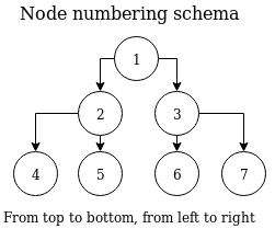
NA directions, inherited categorical levels, predictions and all other information available can be obtained by accessing the corresponding arrays in the same way as shown in case of first_tree.features array. Yet there is one more question to answer - how to find out index of parent node’s left and right child node? There are two arrays left_nodes and right_nodes that fulfill that purpose.
1
2
3
4
first_tree.left_children
[1, 3, 5, -1, -1, -1, -1]
first_tree.right_children
[2, 4, 6, -1, -1, -1, -1]
These two arrays follow the same schema as the rest of these arrays. At index 0, information about root node is to be found. In this case, information about root node’s left child index can be obtained by accessing first_tree.left_children[0]. The output of that operation is 1. This means the index of root node’s left child in all these arrays mentioned is 1. Information about root node’s right child can be obtained in the same way, only the array accessed differs. The result of issuing first_tree.right_children[0] command is 2, which means the index of information root node’s left child in all the arrays available is 2.
Such indices can be then used to fetch information from these arrays directly. For example accessing first_tree.features[2] returns split feature of root node’s right child. Acessing first_tree.left_children[2] returns left child index of root node’s right child.
To demonstrate the above-mentioned capabilities, the following script iterates over all the nodes in the tree, printing only a portion of information available about each node.
1
2
3
4
5
6
7
8
9
10
11
for i in range(0,len(first_tree)):
    print("Node ID {0} has left child node with index {1} and right child node with index {2}. The split feature is {3}."
          .format(first_tree.node_ids[i], first_tree.left_children[i], first_tree.right_children[i], first_tree.features[i]))

Node ID 0 has left child node with index 1 and right child node with index 2. The split feature is Origin.
Node ID 1 has left child node with index 3 and right child node with index 4. The split feature is Origin.
Node ID 2 has left child node with index 5 and right child node with index 6. The split feature is Origin.
Node ID 7 has left child node with index -1 and right child node with index -1. The split feature is None.
Node ID 8 has left child node with index -1 and right child node with index -1. The split feature is None.
Node ID 9 has left child node with index -1 and right child node with index -1. The split feature is None.
Node ID 10 has left child node with index -1 and right child node with index -1. The split feature is None.
Fetching tree with a class
For binomial & multinomial models, a tree class must be specified, as there is a dedicated tree built per each class. The previously built model is a regressional model, therefore a new model must be built. Using the very same dataset and the very same GBM algorithm with exactly the same settings, the explanatory variables are now Origin and Distance. Response variable is set to IsDepDelayed, which only has two values, True and False. Binomial response has a class and thus the class must be specified.
1
2
3
4
5
6
7
8
9
10
11
import h2o
h2o.init()
airlines_data = h2o.import_file("https://s3.amazonaws.com/h2o-airlines-unpacked/allyears2k.csv")
from h2o.estimators import H2OGradientBoostingEstimator
model = H2OGradientBoostingEstimator(ntrees = 3, max_depth = 2)
model.train(x=["Origin", "Distance"], y="IsDepDelayed", training_frame=airlines_data)

from h2o.tree import H2OTree
tree = H2OTree(model = model, tree_number = 0, tree_class = "NO")
print(tree)
Tree related to model GBM_model_python_1541337427535_15. Tree number is 0, tree class is 'NO'
Same approach works for multinomial models. Binomial models have one exception - only one class is considered. In the example above, the class with index 0 is model’s info has been used, which is clas NO.
R Client
As an example dataset, a widely-known Airlines Delay dataset is used. All the example scripts will automatically download the dataset, thus there is no need to download it in advance.
To fetch a tree from a decision tree-based model, it is required to build the model. All the machine learning algorithms with a decision trees as an output are supported. For demonstration purpose, GBM is chosen. It can be found as a function in h2o package as h2o.gbm(...) function. The approach to obtain trees for all the algorithms is exactly the same in R as well. Simply substituting h2o.gbm() model with h2o.randomForest(...), or h2o.xgboost(...) or any other supported algorithm is going to work flawlessly.
Building the example model
Goal is not to produce the best predictor, but an understandable one. Therefore, the example GBM model is very simple. The following script connects H2O R client to H2O backend and imports the Airlines dataset. To keep the model training time at minimum, a maximum number of trees is limited to 3. In order to make the decision tree small and easily understandable, maximum depth of the decision tree is limited to 3. As the tree is binary, this is going to limit the number of nodes to 7. A root node with two children, plus maximum of two children per each of root node’s children. This leads to a total of 7 nodes.
1
2
3
4
require("h2o")
h2o.init()
airlines.data <- h2o.importFile("https://s3.amazonaws.com/h2o-airlines-unpacked/allyears2k.csv")
airlines.model <- h2o.gbm(x = c("Origin"), y = "Distance", training_frame = airlines.data, max_depth = 2, ntrees = 3)
Fetching a basic tree
As the model that is trying to guess the distance of a flight based on flight’s origin is built, the only next step required is to fetch the decision trees behind it. The only next step is to fetch the actual tree. The number of trees in the model has been set to 3 in the H2OGradientBoostingEstimator’s parameters. This means there are three trees to be fetched. When training real models, always watch for early stopping criteria. Having those in place may result in even fewer trees trained than set in the ntrees argument of H2OGradientBoostingEstimator’s constructor.
A tree in H2O’s Python API is represented by a class named H2OTree and is placed in a package h2o.tree. Its fully qualified name is h2o.tree.H2OTree. As a sidenote for Python users also interested in R, the class name H2OTree is shared with R API. An instance of H2OTree represents a single tree related to a single model. If there are n trees built during the training process of a model, then n instances of H2OTree class must be created represent the full set. A tree is fetched by means of H2OTree’s constructor. It takes three arguments:
- Model to fetch the tree from,
- Ordinal number of the tree to fetch
- Class of the tree to fetch
The very first argument is the model. The variable pointing to the GBM model is airlines.model (as shown in the figure above). As the model is training is progressing, multiple trees are built. The second arguments specifies which tree we’d like to build. In Python, indices are numebered from 0, so the index of the first tree is 0 as well. The number of trees has been limited to 3 in the example. For a real-world model, the number of trees behind it can be obtained by accessing the ntrees field of the model, in this case airlines.model@model$model_summary$number_of_trees. The last argument specifies the class of the tree. This argument only applies to categorial response variables. This is not the case of the airlines.model, which has Distance set as a response variable. Distance’s type is numeric, thus the resulting model is a regression and the parameter can be empty. In case of binomial and multinomial models, the class must be specified. Tree classes correspond to the categorical levels of response variable. Fetching of models with categorical response variable is demonstrated in one of the sections below, accompanied with full explanation.
1
airlines.firstTree <- h2o.getModelTree(model = airlines.model, tree_number = 1)
By issuing the commands in the figure above, a tree is fetched and an instance of S4 class H2OTree is created. The tree is related to airlines.model, it is the very first tree created and due to the nature of the problem (regression), there is no tree class specified. Please note the number of the very first tree is 1 and in Python it is zero. In R, indices usually start with 1 and H2O API is aligned to that standard.
Exploring a basic tree
The H2OTree contains all the information available for given tree. A very basic task is to find out how many nodes are there in the tree. Giving the airlins.firstTree as an argument to Python’s built-in len function provides the answer.
1
2
> length(airlines.firstTree)
[1] 7
Another basic task before tree nodes exploration would be printing general description of a tree. To achieve this, give airlines.firstTree as an argument to R’s built-in print function.
1
2
3
> print(airlines.firstTree)
Tree related to model 'GBM_model_R_1541337427535_4'. Tree number is 1, tree class is ''
The tree has 7 nodes
The H2OTree S4 class has a lot of slots:
- left_children,
- right_children,
- node_ids,
- descriptions,
- model_id,
- tree_number,
- tree_class,
- thresholds,
- features,
- levels,
- nas,
- predictions,
- root_node.
The properties tree_number, tree_class and model_id were present in print(airlines.firstTree)’s output. These are related to the tree’s model and together serve a H2OTree's unique identifier. In the next figure, content of those three properties is demonstrated separately.
As mentioned in the introductionary chapter, there are array-like vector structures for fast iteration through the tree. There is also a pre-built tree structure to walk. As every tree begins with a root node, the root_node slot of H2ONode class serves as an entry point to the tree. Besides having several properties to inspect, it also points to its child nodes. Same rules apply to all other nodes when walking down any path in the graph, unless a terminal node is hit. A more detailed introduction to tree walking is available in one of the sub-chapters to follow. All remaining properties of H2OTree are arrays of node properties. With these, iterating through all the nodes in the tree “bottom down, left to right” can be done in O(n), as each index has to be visited only once. This is going to be explained a little bit further as well.
1
2
3
4
5
6
7
8
9
> airlines.firstTree@model_id
[1] "GBM_model_R_1541337427535_4"

> airlines.firstTree@tree_number
[1] 1

> airlines.firstTree@tree_class
# Empty, in case of regression there are no classes
character(0)
Tree inspection using pre-assembled tree structure
There is one special and very powerful property named root_node. This is the beginning of the decision tree that is assembled once the tree is fetched from H2O backend. A root node is in fact an instance of S4 class named H2SplitNode and is naturally the very beginning of all decision paths in graph. It points to its children, which again point to their children, unless an H2OLeafNode is hit. This makes walking the tree very easy both depth-first and breadth-first. For example leaf-node assignments may be transformed to a path through the tree, inspecting each node on the way. Each node provides all the information based on its type. A split node (an instance of H2OSplitNode) contains all the details about the split. A leaf node (an instance of H2OLeafNode) contains information regarding the final prediction made on that node. All nodes may be printed as well.
1
2
3
4
5
6
7
8
9
10
11
> print(airlines.firstTree@root_node)
Node ID 0

Left child node ID = 1
Right child node ID = 2

Splits on column Origin
  - Categorical levels going to the left node: ABE ABQ ACY ALB AMA AVP BDL BGM BHM BIL BOI BTV BUF BUR CAE CHO CHS CLT COS CRP CRW DAL DAY DCA DEN DSM DTW EGE ELP ERI EWR EYW FLL GEG GNV GRR GSO HOU HPN HRL ICT ISP JAN JAX JFK KOA LAN LAS LBB LEX LGA LIH LIT LYH MAF MCI MDT MEM MFR MHT MKE MLB MRY MSP MYR OAK OKC OMA ONT ORF PHF PHL PIT PSP PVD PWM RDU RIC RNO ROA ROC SAT SAV SBN SCK SDF SJC SMF SNA STL SWF SYR TLH TRI TUL TUS TYS UCA
  - Categorical levels to the right node: ANC ATL AUS BNA BOS BWI CLE CMH CVG DFW HNL IAD IAH IND LAX MCO MDW MIA MSY OGG ORD PBI PDX PHX RSW SAN SEA SFO SJU SLC SRQ STT STX TPA

NA values go to the LEFT node
In the figure above, a node has been printed. The information output is always corresponding to the node’s split. If the split is categorical, a complete list of categorical levels corresponding to the node’s split column leading the decision path to the left and to the right is printed. If the split is numerical, the split threshold is printed. If there is a possibility for NA values in given split column to reach the node, the direction of NA values is printed as well. It might as well happen for NA values of a certain column to be diverted onto a different path through the decision tree earlier.
The tree may be walked from the root node all the way until any of the leaf nodes is reached. In the next figure, a “random walk” through the tree is shown. Standing on the root node, a random decision had been made to go to the root node’s left child and then to the right child, which happened to be the leaf node of the chosen path.
1
2
3
4
> airlines.firstTree@root_node@left_child@right_child
Node ID 8

Terminal node. Prediction is -9.453938
A leaf node may also be recognized by it’s class name.
1
2
3
4
5
6
7
> class(airlines.firstTree@root_node@left_child@left_child)
[1] "H2OLeafNode"
attr(,"package")
[1] "h2o"

> class(airlines.firstTree@root_node@left_child@left_child)[1] == "H2OLeafNode"
[1] TRUE
A Split node (H2OSplitNode) is represented by a separate S4 class as well and therefore is easily distinguishable from a Leaf node.
1
2
3
4
5
6
7
> class(airlines.firstTree@root_node)
[1] "H2OSplitNode"
attr(,"package")
[1] "h2o"

> class(airlines.firstTree@root_node)[1] == "H2OSplitNode"
[1] TRUE
Properties of a node may be printed in a human readable format, as demonstrated above. However, the values are still present in node’s properties to process. An H2OSplitNode has the following slots:
- id
- left_child,
- right_child,
- threshold,
- split_feature,
- na_direction,
- left_levels,
- right_levels.
How to access the H2OSplitNode’s slots is demonstrated in the next figure.
1
2
3
4
5
6
7
8
9
10
11
12
13
14
15
16
17
18
19
20
21
22
23
24
25
26
27
28
29
30
31
32
33
34
35
36
37
38
39
40
> airlines.firstTree@root_node@right_child
Node ID 2

Left child node ID = 9
Right child node ID = 10

Splits on column Origin
  - Categorical levels going to the left node: AUS BNA BOS BWI CLE DFW IAD IAH IND LAX MCO MDW MIA MSY ORD PBI PDX PHX RSW SAN SFO SRQ TPA
  - Categorical levels to the right node: ANC ATL CMH CVG HNL OGG SEA SJU SLC STT STX

> airlines.firstTree@root_node@left_child
Node ID 1

Left child node ID = 7
Right child node ID = 8

Splits on column Origin
  - Categorical levels going to the left node: ABE ABQ ACY ALB AMA AVP BDL BGM BIL BTV BUF BUR CAE CHO CHS CRP CRW DAL DAY DCA DSM EGE ELP ERI EYW GNV GRR GSO HPN HRL ICT JFK KOA LAN LBB LEX LIH LYH MAF MDT MFR MKE MLB MRY MYR OAK OKC OMA ONT ORF PHF PSP PVD PWM RDU RIC RNO ROA ROC SAV SBN SCK SNA SWF SYR TLH TRI TUL TYS UCA
  - Categorical levels to the right node: BHM BOI CLT COS DEN DTW EWR FLL GEG HOU ISP JAN JAX LAS LGA LIT MCI MEM MHT MSP PHL PIT SAT SDF SJC SMF STL TUS

NA values go to the RIGHT node

> airlines.firstTree@root_node@threshold
[1] NA

> airlines.firstTree@root_node@split_feature
[1] "Origin"

> airlines.firstTree@root_node@na_direction
[1] "LEFT"

> airlines.firstTree@root_node@left_levels
 [1] "ABE" "ABQ" "ACY" "ALB" "AMA" "AVP" "BDL" "BGM" "BHM" "BIL" "BOI" "BTV" "BUF" "BUR" "CAE" "CHO" "CHS" "CLT" "COS" "CRP" "CRW" "DAL" "DAY" "DCA" "DEN" "DSM" "DTW" "EGE" "ELP" "ERI" "EWR"
[32] "EYW" "FLL" "GEG" "GNV" "GRR" "GSO" "HOU" "HPN" "HRL" "ICT" "ISP" "JAN" "JAX" "JFK" "KOA" "LAN" "LAS" "LBB" "LEX" "LGA" "LIH" "LIT" "LYH" "MAF" "MCI" "MDT" "MEM" "MFR" "MHT" "MKE" "MLB"
[63] "MRY" "MSP" "MYR" "OAK" "OKC" "OMA" "ONT" "ORF" "PHF" "PHL" "PIT" "PSP" "PVD" "PWM" "RDU" "RIC" "RNO" "ROA" "ROC" "SAT" "SAV" "SBN" "SCK" "SDF" "SJC" "SMF" "SNA" "STL" "SWF" "SYR" "TLH"
[94] "TRI" "TUL" "TUS" "TYS" "UCA"

> airlines.firstTree@root_node@right_levels
 [1] "ANC" "ATL" "AUS" "BNA" "BOS" "BWI" "CLE" "CMH" "CVG" "DFW" "HNL" "IAD" "IAH" "IND" "LAX" "MCO" "MDW" "MIA" "MSY" "OGG" "ORD" "PBI" "PDX" "PHX" "RSW" "SAN" "SEA" "SFO" "SJU" "SLC" "SRQ"
[32] "STT" "STX" "TPA"
A leaf node (type H2OLeafNode) lacks the properties regarding column split, but contains a prediction-related information instead:
- id,
- prediction.
Access to H2OLeafNode’s properties is demonstrated in the next figure.
1
2
3
4
> airlines.firstTree@root_node@left_child@right_child@id
[1] 8
> airlines.firstTree@root_node@left_child@right_child@prediction
[1] -9.453938
Iteration throught node-info vectors(arrays)
A second way to obtain iformation about tree’s nodes are vectors built-in to H2OTree object type. First, there are multiple vectors. Each vector holds different kind of information about nodes.
- left_children holds indices of node’s left child,
- right_children holds indices of node’s right child,
- node_ids provides node’s unique identifier inside H2O (may differ from index),
- descriptions holds a human-readable description of each node,
- thresholds provide split threshold for each node,
- features vector tells which feature is used for split on given node ,
- levels show list of categorical levels inherited by each node from parent (if any),
- nas vector holds information about NA value direction (left node, right node, none/unavailable),
- predictions provides information about prediction on given nodes (if applicable).
Length of these vectors alway equals to the number of nodes in the tree. By iterating from 0 to len(tree), all the information available can be extracted. As each node is visited only once, the complexity of this task is O(n). As there are multiple vectors, only those holding the information required may be accessed.
1
2
3
4
> length(airlines.firstTree)
[1] 7
> length(airlines.firstTree@left_children)
[1] 7
In the following example, a vector of split features is printed. Each index represents a node and a feature the node splits on. If the value is None, the node is terminal. As there is only one feature in the example model named Origin, all the split features are the same. As the depth of the tree is limited to 3, the vector below makes perfect sense. Index 1 is the root node and it splits on feature Origin. As the tree is binary, root node has two child nodes with index 2 and 3. Both of root node’s children also have child nodes and thus have a split feature assigned. In this case it is Origin again. If the first_tree.features vector is accessed at indices 1, 2 and 3, the vector says exactly what has been stated above - the split features are Origin. The two of root node’s children also have child nodes - leaf nodes. Sometimes referred to as terminal nodes. These node do not have any children, but represent the final prediction made. There are four of them, as the graph is binary and root node has two child nodes, each having two child leaf nodes. As there is not split available, the split value is None.
1
2
> airlines.firstTree@features
[1] "Origin" "Origin" "Origin" NA       NA       NA       NA
The example above raises one important question - how are node indices numbered? Nodes are always numbered from the top of the tree down to the lowest level, from left to right. This is demonstrated in the following diagram. This corresponds with the example above - root node having two child nodes, plus four leaf nodes at depth = 3 (assuming root node depth = 1).
NA directions, inherited categorical levels, predictions and all other information available can be obtained by accessing the corresponding vectors in the same way as shown in case of first_tree.features vector. Yet there is one more question to answer - how to find out index of parent node’s left and right child node? There are two vectors left_nodes and right_nodes that fulfill that purpose.
1
2
3
4
> airlines.firstTree@left_children
[1]  1  3  5 -1 -1 -1 -1
> airlines.firstTree@right_children
[1]  2  4  6 -1 -1 -1 -1
These two vectors follow the same schema as the rest of the other vectors. At index 1, information about root node is to be found. In this case, information about root node’s left child index can be obtained by accessing first_tree.left_children[1]. The output of that operation is 2. This means the index of root node’s left child in all these vectors mentioned is 2. Information about root node’s right child can be obtained in the same way, only the vectors accessed differs. The result of issuing first_tree.right_children[1] command is 3, which means the index of information root node’s left child in all the vectors available is 3.
Such indices can be then used to fetch information from these vectors directly. For example accessing first_tree.features[3] returns split feature of root node’s right child. Acessing first_tree.left_children[3] returns left child index of root node’s right child.
To demonstrate the above-mentioned capabilities, the following script iterates over all the nodes in the tree, printing only a portion of information available about each node.
1
2
3
4
5
6
7
8
9
10
11
12
> for (i in 1:length(airlines.firstTree)){
+     info <- sprintf("Node ID %s has left child node with index %s and right child node with index %s. The split feature is %s",
+             airlines.firstTree@node_ids[i], airlines.firstTree@left_children[i], airlines.firstTree@right_children[i], airlines.firstTree@features[i])
+     print(info)
+ }
[1] "Node ID 0 has left child node with index 1 and right child node with index 2. The split feature is Origin"
[1] "Node ID 1 has left child node with index 3 and right child node with index 4. The split feature is Origin"
[1] "Node ID 2 has left child node with index 5 and right child node with index 6. The split feature is Origin"
[1] "Node ID 7 has left child node with index -1 and right child node with index -1. The split feature is NA"
[1] "Node ID 8 has left child node with index -1 and right child node with index -1. The split feature is NA"
[1] "Node ID 9 has left child node with index -1 and right child node with index -1. The split feature is NA"
[1] "Node ID 10 has left child node with index -1 and right child node with index -1. The split feature is NA"
Fetching tree with a class
For binomial & multinomial models, a tree class must be specified, as there is a dedicated tree built per each class. The previously built model is a regressional model, therefore a new model must be built. Using the very same dataset and the very same GBM algorithm with exactly the same settings, the explanatory variables are now Origin and Distance. Response variable is set to IsDepDelayed, which only has two values, True and False. Binomial response has a class and thus the class must be specified.
1
2
3
4
5
require("h2o")
h2o.init()
airlines.data = h2o.importFile("https://s3.amazonaws.com/h2o-airlines-unpacked/allyears2k.csv")
airlines.model = h2o.gbm(x = c("Origin", "Distance"), y = "IsDepDelayed", training_frame = airlines.data, max_depth = 2, ntrees = 3)
h2o.getModelTree(model = airlines.model, tree_number = 1, tree_class = "NO") # Class is specified, response is binomial
Same approach works for multinomial models. Binomial models have one exception - only one class is considered. In the example above, the class with index 0 is model’s info has been used, which is clas NO.
Java API
This section is for developers and expert users implementing functionality directly relying. When trees are fetched, H2O’s endpoint named /3/Tree is called. The request and response format is described by the TreeV3 class. Request handling logic is contained in the TreeHandler class.
When H2OTree is constructed, H2O backend provides the tree structure to the client in a semi-compressed format and the client builds the represenation. This reduces the amount of data transferred and delegates the easy task of tree assembly to the client, making all the resources on the backend immediately available.
Please note the API may undergo changes in future and is not aimed to be used directly.
Future plans & Credits
Currently, the information about decision trees are available. But the development doesn’t end here. Makers are always gonna make. Plan for the future is to enrich this functionality to provide direct support of most common use-cases of our new API. In order to do that, user feedback must be gathered first. Development of H2O is open & public, you can always contact us on Gitter or suggest new features in JIRA. As even the development process is open, H2O always welcomes new contributions into our H2O-3 GitHub repository. If you ever feel like having a good addition to our API, fork the repository, create a pull request and H2O will handle the rest. At H2O, we care about our community and care about feedback of our users. If there is functionality missing, or some part of the API is misbehaving, please contact us.
The API described is a team work. From design and implementation to never-ending enhancements. The following makers made it possible: Michal Kurka, Erin LeDell, Angela Bartz, Wendy Wong, Petr Kozelka, Lauren DiPerna, Jakub Hava, Pavel Pscheidl.